A Short Introduction to splines2

Wenjie Wang

2024-09-02

Introduction

The R package splines2 is intended to be a user-friendly supplementary package to the base package splines. It provides functions to construct a variety of regression spline basis functions that are not available from splines. Most functions have a very similar user interface with the function splines::bs(). More specifically, splines2 allows users to construct the basis functions of

• B-splines
• M-splines
• I-splines
• C-splines
• periodic splines
• natural cubic splines
• generalized Bernstein polynomials

along with their integrals (except C-splines) and derivatives of given order by closed-form recursive formulas.

Compared to splines, the package splines2 provides convenient interfaces for spline derivatives with consistent handling on NA’s. Most of the implementations are in C++ with the help of Rcpp and RcppArmadillo since v0.3.0, which boosted the computational performance.

In the remainder of this vignette, we illustrate the basic usage of most functions in the package through examples. We refer readers to Wang and Yan (2021) for a more formal introduction to the package with applications to shape-restricted regression. See the package manual for more details about function usage.

library(splines2)
packageVersion("splines2")

## [1] '0.5.3'

B-splines

B-spline Basis Functions

The bSpline() function generates the basis matrix for B-splines and extends the function bs() of the package splines by providing 1) the piece-wise constant basis functions when degree = 0, 2) the derivatives of basis functions for a positive derivs, 3) the integrals of basis functions if integral = TRUE, 4) periodic basis functions based on B-splines if periodic = TRUE.

One example of linear B-splines with three internal knots is as follows:

knots <- c(0.3, 0.5, 0.6)
x <- seq(0, 1, 0.01)
bsMat <- bSpline(x, knots = knots, degree = 1, intercept = TRUE)
plot(bsMat, mark_knots = "all")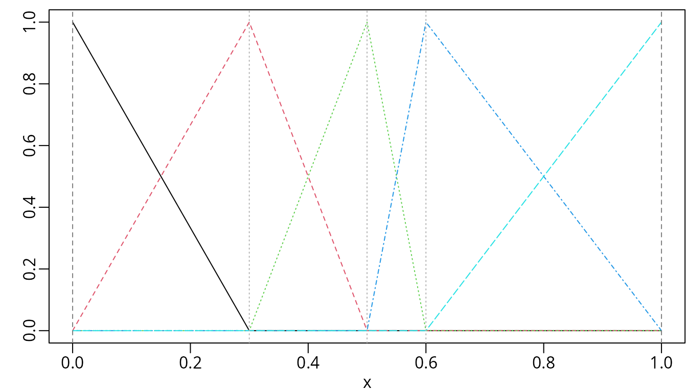

B-splines of degree one with three internal knots placed at 0.3, 0.5, and 0.6.

Integrals and Derivatives of B-splines

For convenience, the package also provides functions ibs() and dbs() for constructing the B-spline integrals and derivatives, respectively. Two toy examples are as follows:

ibsMat <- ibs(x, knots = knots, degree = 1, intercept = TRUE)
op <- par(mfrow = c(1, 2))
plot(bsMat, mark_knots = "internal")
plot(ibsMat, mark_knots = "internal")
abline(h = c(0.15, 0.2, 0.25), lty = 2, col = "gray")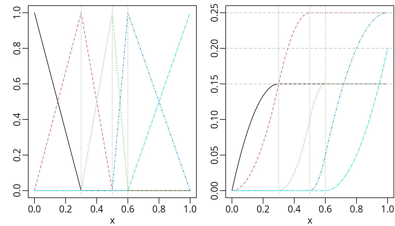

Piecewise linear B-splines (left) and their integrals (right).

bsMat <- bSpline(x, knots = knots, intercept = TRUE)
dbsMat <- dbs(x, knots = knots, intercept = TRUE)
plot(bsMat, mark_knots = "internal")
plot(dbsMat, mark_knots = "internal")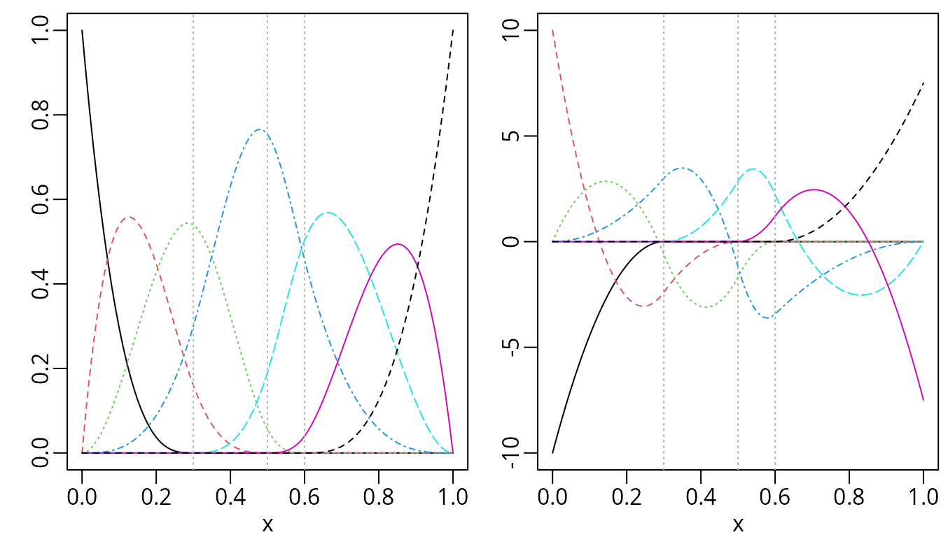

Cubic B-spline (left) and their first derivative (right).

We may also obtain the derivatives easily by the deriv() method as follows:

is_equivalent <- function(a, b) {
    all.equal(a, b, check.attributes = FALSE)
}
stopifnot(is_equivalent(dbsMat, deriv(bsMat)))

Periodic B-splines

The function bSpline() produces periodic spline basis functions following Piegl and Tiller (1997, chap. 12) when periodic = TRUE is specified. Different from the regular basis functions, the x is allowed to be placed outside the boundary and the Boundary.knots defines the cyclic interval. For instance, one may obtain the periodic cubic B-spline basis functions with cyclic interval (0, 1) as follows:

px <- seq(0, 3, 0.01)
pbsMat <- bSpline(px, knots = knots, Boundary.knots = c(0, 1),
                  intercept = TRUE, periodic = TRUE)
ipMat <- ibs(px, knots = knots, Boundary.knots = c(0, 1),
             intercept = TRUE, periodic = TRUE)
dp1Mat <- deriv(pbsMat)
dp2Mat <- deriv(pbsMat, derivs = 2)
par(mfrow = c(1, 2))
plot(pbsMat, ylab = "Periodic B-splines", mark_knots = "boundary")
plot(ipMat, ylab = "The integrals", mark_knots = "boundary")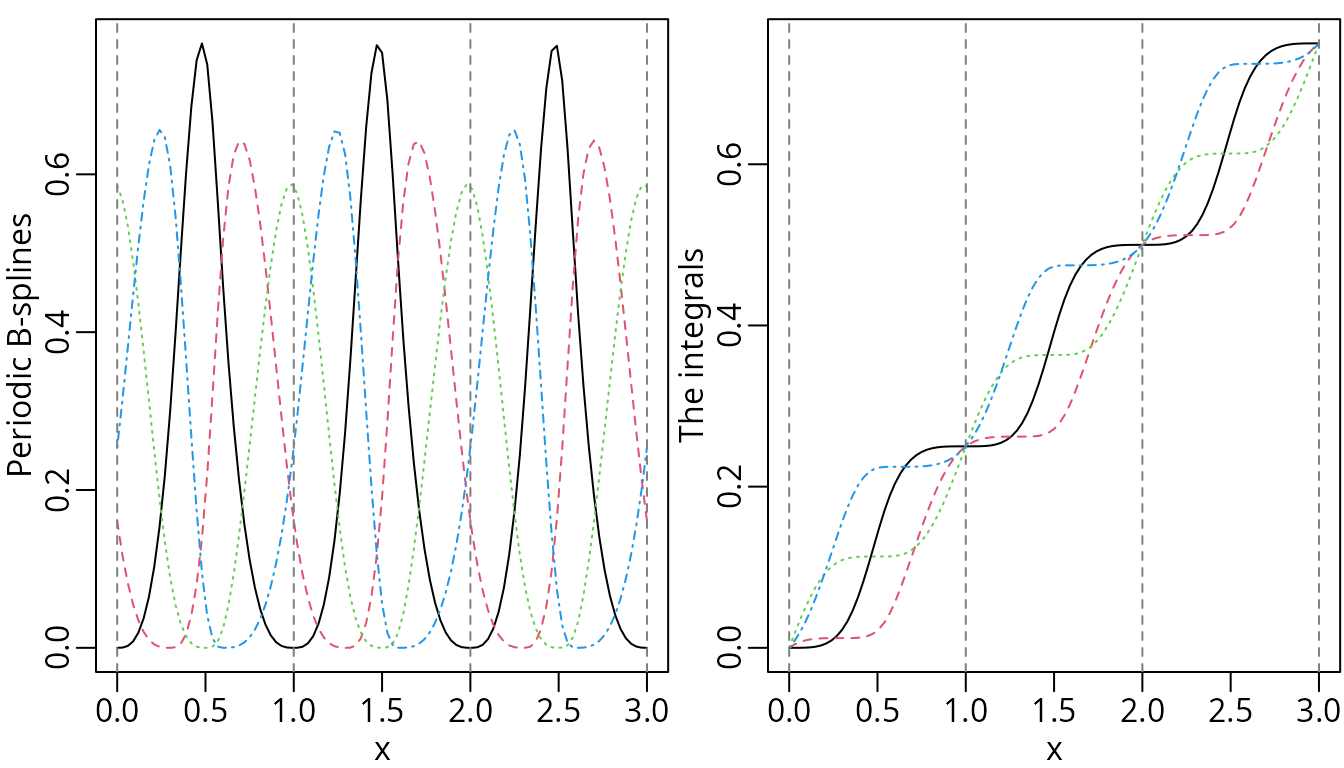

plot(dp1Mat, ylab = "The 1st derivatives", mark_knots = "boundary")
plot(dp2Mat, ylab = "The 2nd derivatives", mark_knots = "boundary")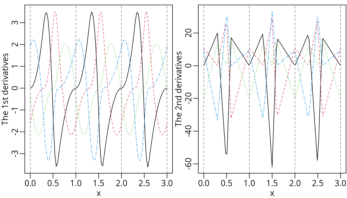

For reference, the corresponding integrals and derivatives are also visualized.

M-Splines

M-spline Basis Functions

M-splines (Ramsay 1988) can be considered the normalized version of B-splines with unit integral within boundary knots. An example given by Ramsay (1988) was a quadratic M-splines with three internal knots placed at 0.3, 0.5, and 0.6. The default boundary knots are the range of x, and thus 0 and 1 in this example.

msMat <- mSpline(x, knots = knots, degree = 2, intercept = TRUE)
par(op)
plot(msMat, mark_knots = "all")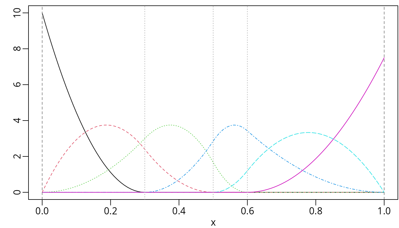

Quadratic M-spline with three internal knots placed at 0.3, 0.5, and 0.6.

The derivative of the given order of M-splines can be obtained by specifying a positive integer to argument dervis of mSpline(). Similarly, for an existing mSpline object generated by mSpline(), one can use the deriv() method for derivaitives. For example, the first derivative of the M-splines given in the previous example can be obtained equivalently as follows:

dmsMat1 <- mSpline(x, knots = knots, degree = 2, intercept = TRUE, derivs = 1)
dmsMat2 <- deriv(msMat)
stopifnot(is_equivalent(dmsMat1, dmsMat2))

Periodic M-Splines

The mSpline() function produces periodic splines based on M-spline basis functions when periodic = TRUE is specified. The Boundary.knots defines the cyclic interval, which is the same with the periodic B-splines.

pmsMat <- mSpline(px, knots = knots, intercept = TRUE,
                  periodic = TRUE, Boundary.knots = c(0, 1))
plot(pmsMat, ylab = "Periodic Basis", mark_knots = "boundary")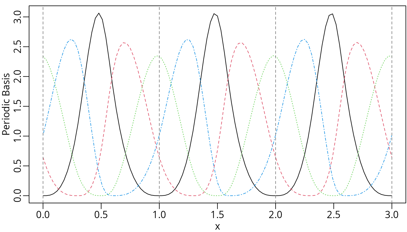

Cubic periodic M-splines.

We may still specify the argument derivs in mSpline() or use the corresponding deriv() method to obtain the derivatives when periodic = TRUE.

dpmsMat <- deriv(pmsMat)
plot(dpmsMat, ylab = "The 1st derivatives", mark_knots = "boundary")

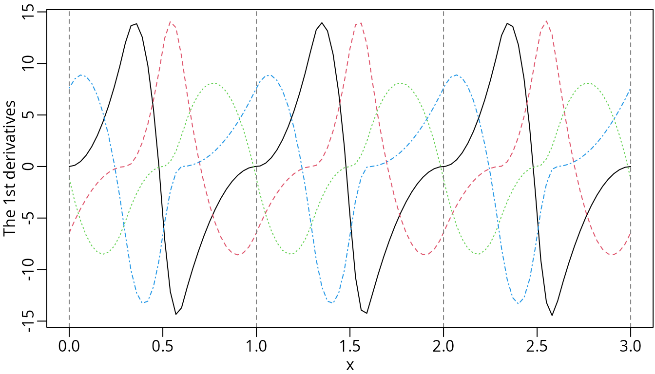
The first derivatives of the periodic M-splines.

Furthermore, we can obtain the integrals of the periodic M-splines by specifying integral = TRUE. The integral is integrated from the left boundary knot.

ipmsMat <- mSpline(px, knots = knots, intercept = TRUE,
                   periodic = TRUE, Boundary.knots = c(0, 1), integral = TRUE)
plot(ipmsMat, ylab = "Integrals", mark_knots = "boundary")
abline(h = seq.int(0, 3), lty = 2, col = "gray")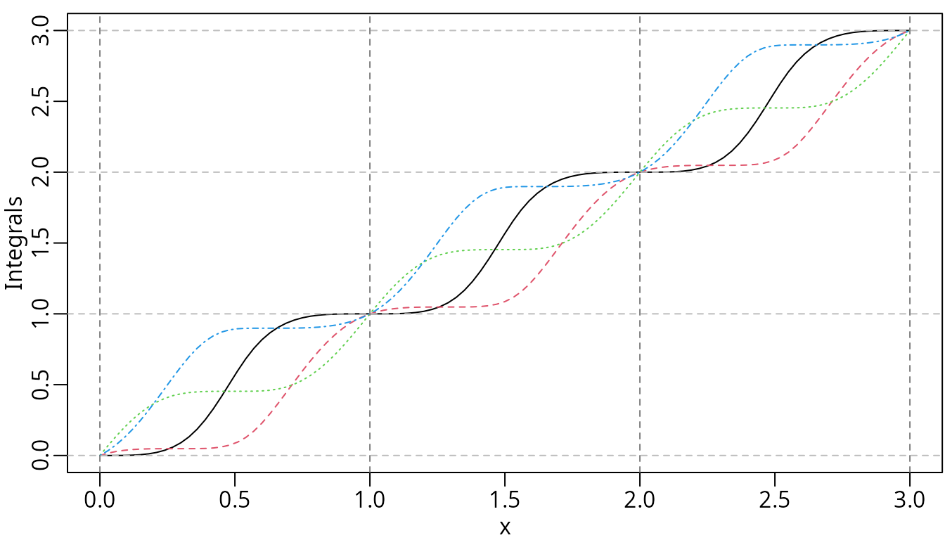

The integrals of the periodic M-splines.

I-Splines

I-splines (Ramsay 1988) are simply the integral of M-splines and thus monotonically nondecreasing with unit maximum value. A monotonically nondecreasing (nonincreasing) function can be fitted by a linear combination of I-spline basis functions with nonnegative (nonpositive) coefficients plus a constant, where the coefficient of the constant is unconstrained.

The example given by Ramsay (1988) was the I-splines corresponding to the quadratic M-splines with three internal knots placed at 0.3, 0.5, and 0.6. Notice that the degree of I-splines is defined from the associated M-splines instead of their polynomial degree.

isMat <- iSpline(x, knots = knots, degree = 2, intercept = TRUE)
plot(isMat, mark_knots = "internal")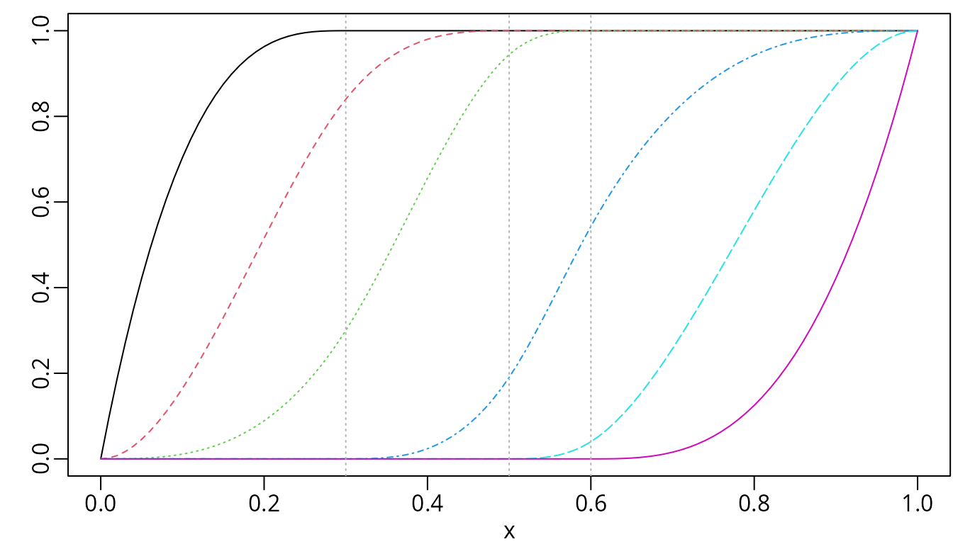

I-splines of degree two with three internal knots placed at 0.3, 0.5, and 0.6.

The corresponding M-spline basis matrix can be obtained easily as the first derivatives of the I-splines by the deriv() method.

stopifnot(is_equivalent(msMat, deriv(isMat)))

We may specify derivs = 2 in the deriv() method for the second derivatives of the I-splines, which are equivalent to the first derivatives of the corresponding M-splines.

dmsMat3 <- deriv(isMat, 2)
stopifnot(is_equivalent(dmsMat1, dmsMat3))

C-Splines

Convex splines (Meyer 2008) called C-splines are scaled integrals of I-splines with unit maximum value at the right boundary knot. Meyer (2008) applied C-splines to shape-restricted regression analysis. The monotone (nondecreasing) property of I-spines ensures the convexity of C-splines. A convex regression function can be estimated using linear combinations of the C-spline basis functions with nonnegative coefficients, plus an unconstrained linear combination of a constant and an identity function $g(x)=x$. If the underlying regression function is both increasing and convex, the coefficient on the identity function is restricted to be nonnegative as well.

We may specify the argument scale = FALSE in the function cSpline() to disable the scaling of the integrals of I-splines. Then the actual integrals of the corresponding I-splines will be returned. If scale = TRUE (by default), each C-spline basis is scaled to have unit height at the right boundary knot.

csMat1 <- cSpline(x, knots = knots, degree = 2, intercept = TRUE)
plot(csMat1)
abline(h = 1, v = knots, lty = 2, col = "gray")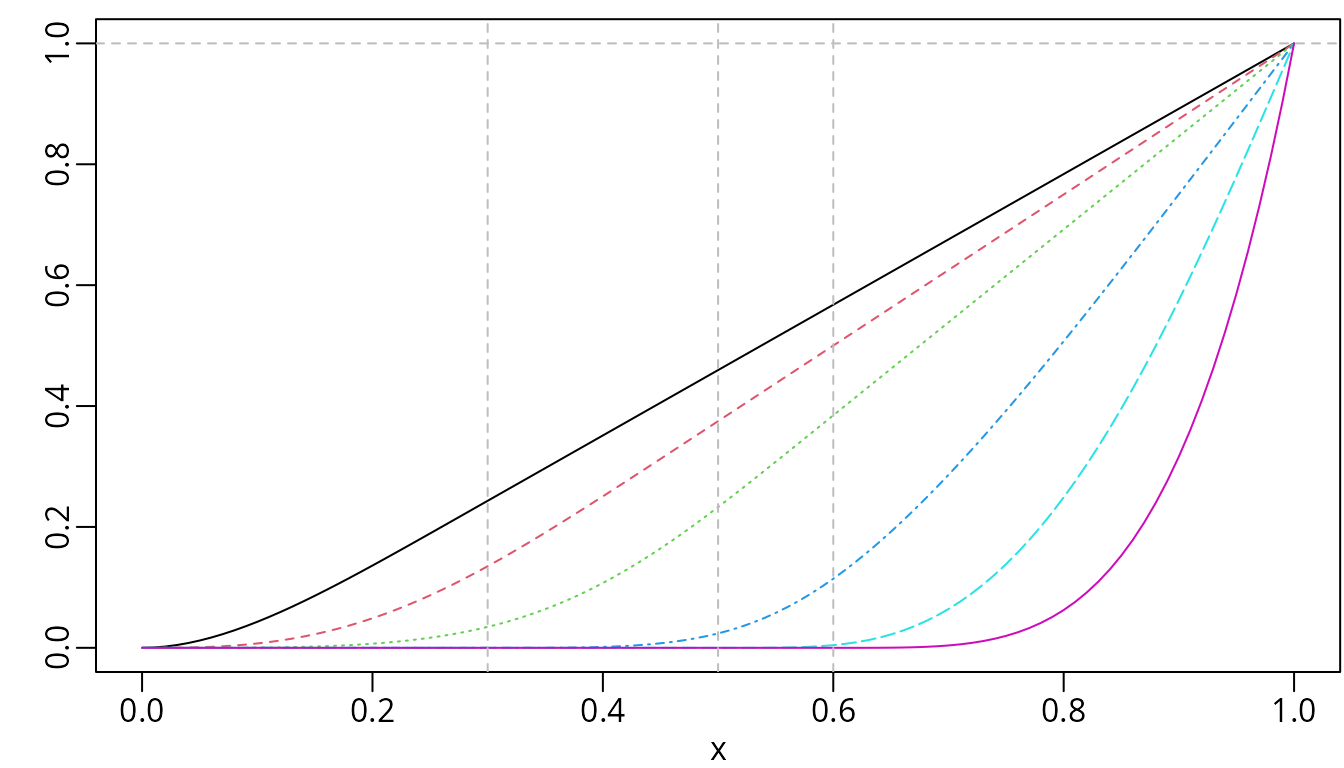

C-splines of degree two with three internal knots placed at 0.3, 0.5, and 0.6.

Similarly, the deriv() method can be used to obtain the derivatives. A nested call of deriv() is supported for derivatives of a higher order. However, the argument derivs of the deriv() method can be specified directly for better computational performance. For example, the first and second derivatives can be obtained by the following equivalent approaches, respectively.

csMat2 <- cSpline(x, knots = knots, degree = 2, intercept = TRUE, scale = FALSE)
stopifnot(is_equivalent(isMat, deriv(csMat2)))
stopifnot(is_equivalent(msMat, deriv(csMat2, 2)))
stopifnot(is_equivalent(msMat, deriv(deriv(csMat2))))

Generalized Bernstein Polynomials

The Bernstein polynomials are equivalent to B-splines without internal knots and have also been applied to shape-constrained regression analysis (e.g., Wang and Ghosh 2012). The $i$-th basis of the generalized Bernstein polynomials of degree $n$ over $[a, b]$ is defined as follows: $$B_i^n(x)=\frac{1}{(b-a)^n}{n\choose i}(x-a)^i (b-x)^{n-i},~i\in\{0,\ldots,n\},$$ where $a\le x\le b$. It reduces to regular Bernstein polynomials defined over $[0, 1]$ when $a = 0$ and $b = 1$.

We may obtain the basis matrix of the generalized using the function bernsteinPoly(). For example, the Bernstein polynomials of degree 4 over $[0, 1]$ and is generated as follows:

x1 <- seq.int(0, 1, 0.01)
x2 <- seq.int(- 1, 1, 0.01)
bpMat1 <- bernsteinPoly(x1, degree = 4, intercept = TRUE)
bpMat2 <- bernsteinPoly(x2, degree = 4, intercept = TRUE)
par(mfrow = c(1, 2))
plot(bpMat1)
plot(bpMat2)

Bernstein polynomials of degree 4 over [0, 1] (left) and the generalized version over [- 1, 1] (right).

In addition, we may specify integral = TRUE or derivs = 1 in bernsteinPoly() for their integrals or first derivatives, respectively.

ibpMat1 <- bernsteinPoly(x1, degree = 4, intercept = TRUE, integral = TRUE)
ibpMat2 <- bernsteinPoly(x2, degree = 4, intercept = TRUE, integral = TRUE)
dbpMat1 <- bernsteinPoly(x1, degree = 4, intercept = TRUE, derivs = 1)
dbpMat2 <- bernsteinPoly(x2, degree = 4, intercept = TRUE, derivs = 1)
par(mfrow = c(2, 2))
plot(ibpMat1, ylab = "Integrals")
plot(ibpMat2, ylab = "Integrals")
plot(dbpMat1, ylab = "Derivatives")
plot(dbpMat2, ylab = "Derivatives")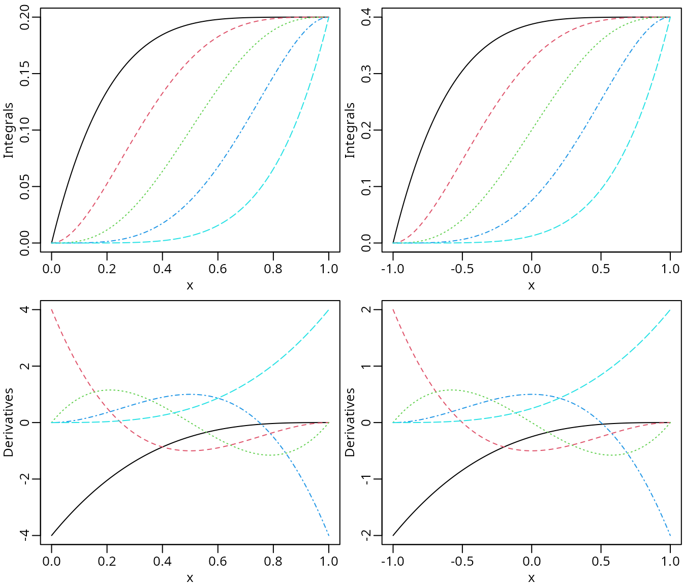

The integrals (upper panel) and the first derivatives (lower panel) of Bernstein polynomials of degree 4.

Similarly, we may also use the deriv() method to get derivatives of an existing bernsteinPoly object.

stopifnot(is_equivalent(dbpMat1, deriv(bpMat1)))
stopifnot(is_equivalent(dbpMat2, deriv(bpMat2)))
stopifnot(is_equivalent(dbpMat1, deriv(ibpMat1, 2)))
stopifnot(is_equivalent(dbpMat2, deriv(ibpMat2, 2)))

Natural Cubic Splines

Nonnegative Natural Cubic Basis Functions

The package provides two variants of the natural cubic splines that can be constructed by naturalSpline() and nsk(), respectively, both of which are different from splines::ns().

The naturalSpline() function returns nonnegative basis functions (within the boundary) for natural cubic splines by utilizing a closed-form null space derived from the second derivatives of cubic B-splines. When integral = TRUE, the function naturalSpline() returns the integral of each natural spline basis.

nsMat <- naturalSpline(x, knots = knots, intercept = TRUE)
insMat <- naturalSpline(x, knots = knots, intercept = TRUE, integral = TRUE)
par(mfrow = c(1, 2))
plot(nsMat, ylab = "Basis")
plot(insMat, ylab = "Integrals")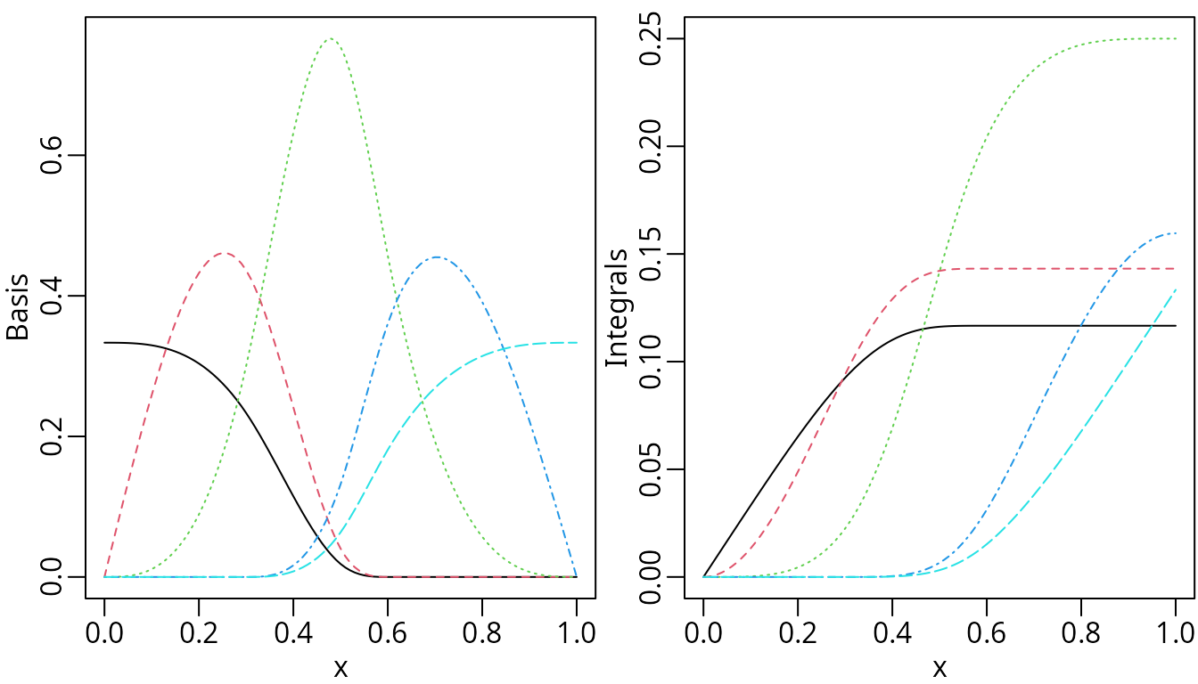

Nonnegative natural cubic splines (left) and corresponding integrals (right).

stopifnot(is_equivalent(nsMat, deriv(insMat)))

Similarly, one may directly specify the argument derivs in naturalSpline() or use the corresponding deriv() method to obtain the derivatives of spline basis functions.

d1nsMat <- naturalSpline(x, knots = knots, intercept = TRUE, derivs = 1)
d2nsMat <- deriv(nsMat, 2)
matplot(x, d1nsMat, type = "l", ylab = "The 1st derivatives")
matplot(x, d2nsMat, type = "l", ylab = "The 2nd derivatives")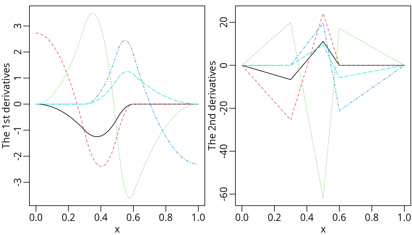

The derivatives of natural cubic splines.

Natural Cubic Basis Functions with Unit Heights at Knots

The function nsk() produces another variant of natural cubic splines, where only one of the spline basis functions is nonzero with unit height at every boundary and internal knot. As a result, the coefficients of the basis functions are the values of the spline function at the knots, which makes it more straightforward to interpret the coefficient estimates. This idea originated from the function nsk() of the survival package (introduced in version 3.2-8). The implementation of the nsk() of splines2 essentially follows the survival::nsk() function. One noticeable argument for nsk() is trim (equivalent to the argument b of survival::nsk()). One may specify trim = 0.05 to exclude 5% of the data from both sides when setting the boundary knots, which can be a more sensible choice in practice due to possible outliers. The trim argument is also available for naturalSpline(), which however is zero by default for backward compatibility. An illustration of the basis functions generated by nsk() is as follows:

nskMat <- nsk(x, knots = knots, intercept = TRUE)
par(op)
plot(nskMat, ylab = "nsk()", mark_knots = "all")
abline(h = 1, col = "red", lty = 3)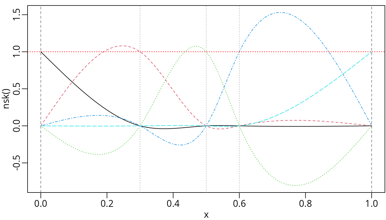

We can visually verify that only one basis function takes a value of one at each knot.

Helper and Alias Functions

Update Spline’s Specification by update()

The update() function is an S3 method to generate spline basis functions with new x, degree, knots, or df specifications. The first argument is an existing splines2 object and additional named arguments will be passed to the corresponding functions to update the spline basis functions. Suppose we want to add two more knots to nskMat for natural cubic spline basis functions and exclude 5% of the data from both sides in total when placing the boundary knots. We can utilize the update() method as follows:

nskMat2 <- update(nskMat, knots = c(knots, 0.2, 0.4), trim = 0.025)
knots(nskMat2)

## [1] 0.2 0.3 0.4 0.5 0.6

stopifnot(all.equal(quantile(x, c(0.025, 0.975), names = FALSE),
                    knots(nskMat2, "boundary")))

Evaluation by predict()

The predict() method for splines2 objects allows one to evaluate the spline function if a coefficient vector is specified via the coef argument. In addition, it internally calls the update() method to update the basis functions before computing the spline function, which can be useful to get the derivatives of the spline function. If the coef argument is not specified, the predict() method will be equivalent to the update() method. For instance, we can compute the first derivative of the I-spline function from the previous example with a coefficient vector seq(0.1, by = 0.1, length.out = ncol(isMat)) at $x = (0.275, 0.525, 0.8)$ as follows:

new_x <- c(0.275, 0.525, 0.8)
names(new_x) <- paste0("x=", new_x)
(isMat2 <- predict(isMat, newx = new_x)) # the basis functions at new x

##                 1         2         3         4        5     6
## x=0.275 0.9994213 0.7730556 0.2310764 0.0000000 0.000000 0.000
## x=0.525 1.0000000 1.0000000 0.9765625 0.2696429 0.000625 0.000
## x=0.8   1.0000000 1.0000000 1.0000000 0.9428571 0.580000 0.125

stopifnot(all.equal(predict(isMat, newx = new_x), update(isMat, x = new_x)))
## compute the first derivative of the I-spline function in different ways
beta <- seq(0.1, by = 0.1, length.out = ncol(isMat))
deriv_ispline1 <- predict(isMat, newx = new_x, coef = beta, derivs = 1)
deriv_ispline2 <- predict(update(isMat, x = new_x, derivs = 1), coef = beta)
deriv_ispline3 <- c(predict(deriv(isMat), newx = new_x) %*% beta)
stopifnot(all.equal(deriv_ispline1, deriv_ispline2))
stopifnot(all.equal(deriv_ispline2, deriv_ispline3))

Visualization by plot()

As one may notice in the previous examples, we may visualize the spline basis functions easily with the plot() method. By default, the spline basis functions are visualized at 101 equidistant grid points within the range of x, which can be tweaked by arguments from, to, and n. In addition, we can indicate the placement of knots by vertical lines through the argument mark_knots. The available options are "none", "internal", "boundary", and "all". A fitted spline function can be visualized by specifying the argument coef. An example of nsk() is as follows:

beta <- seq.int(0.2, length.out = ncol(nskMat), by = 0.2)
plot(nskMat, ylab = "nsk()", mark_knots = "all", coef = beta)
abline(h = beta, col = seq_along(beta), lty = 3)

Including Spline Basis Functions in Model Formulas

It is common to directly include spline basis functions in a model formula. To avoid a lengthy model formula, the package provides alias functions that are summarized in the following table:

Function	Equivalent Alias
bSpline()	bsp()
mSpline()	msp()
iSpline()	isp()
cSpline()	csp()
bernsteinPoly()	bpoly()
naturalSpline()	nsp()

One may create new alias functions. For example, we can create a new alias function simply named b() for B-splines and obtain equivalent models as follows:

b <- bSpline # create an alias for B-splines
mod1 <- lm(weight ~ b(height, degree = 1, df = 3), data = women)
iknots <- with(women, knots(bSpline(height, degree = 1, df = 3)))
mod2 <- lm(weight ~ bSpline(height, degree = 1, knots = iknots), data = women)
pred1 <- predict(mod1, head(women, 10))
pred2 <- predict(mod2, head(women, 10))
stopifnot(all.equal(pred1, pred2))

Nevertheless, there is a possible pitfall when using a customized wrapper function for spline basis functions along with a data-dependent placement of knots. When we make model predictions for a given new data, the placement of the internal/boundary knots can be different from the original placement that depends on the training set. As a result, the spline basis functions generated for prediction may not be the same as the counterparts used in the model fitting. A simple example is as follows:

## generates quadratic spline basis functions based on log(x)
qbs <- function(x, ...) {
    splines2::bSpline(log(x), ..., degree = 2)
}
mod3 <- lm(weight ~ qbs(height, df = 5), data = women)
mod4 <- lm(weight ~ bsp(log(height), degree = 2, df = 5), data = women)
stopifnot(all.equal(unname(coef(mod3)), unname(coef(mod4)))) # the same coef
pred3 <- predict(mod3, head(women, 10))
pred4 <- predict(mod4, head(women, 10))
all.equal(pred3, pred4)

## [1] "Mean relative difference: 0.07185939"

pred0 <- predict(qbs(women$height, df = 5),
                 newx = head(log(women$height), 10),
                 coef = coef(mod3)[- 1]) + coef(mod3)[1]
stopifnot(all.equal(pred0, pred4, check.names = FALSE))

Although the coefficient estimates are the same, the prediction results by using the predict.lm() differ. Using an alias function in the model formula produces correct results.

To resolve this issue, we can create an S3 method for stats::makepredictcall() as follows:

## generates quadratic spline basis functions based on log(x) with a new class
qbs <- function(x, ...) {
    res <- splines2::bSpline(log(x), ..., degree = 2)
    class(res) <- c("qbs", class(res))
    return(res)
}
## a utility to help model.frame() create the right matrices
makepredictcall.qbs <- function(var, call) {
    if (as.character(call)[1L] == "qbs" ||
    (is.call(call) && identical(eval(call[[1L]]), qbs))) {
        at <- attributes(var)[c("knots", "Boundary.knots", "intercept",
                                "periodic", "derivs", "integral")]
        call <- call[1L:2L]
        call[names(at)] <- at
    }
    call
}
## the same example
mod3 <- lm(weight ~ qbs(height, df = 5), data = women)
mod4 <- lm(weight ~ bsp(log(height), degree = 2, df = 5), data = women)
stopifnot(all.equal(unname(coef(mod3)), unname(coef(mod4)))) # the same coef
pred3 <- predict(mod3, head(women, 10))
pred4 <- predict(mod4, head(women, 10))
all.equal(pred3, pred4) # should be TRUE this time

## [1] TRUE

Extract Specifications by $

The basis specifications are saved as attributes of the returned splines2 objects, which means that we can extract one of the specifications by attr(). Alternatively, we can treat splines2 objects as lists and use the corresponding $ method. For example, it is straightforward to extract the specified trim of nskMat2 by attr(nskMat2, "trim") or simply nskMat2$trim.

c(nskMat2$trim, attr(nskMat2, "trim"))

## [1] 0.025 0.025

Reference

Meyer, Mary C. 2008. “Inference Using Shape-Restricted Regression Splines.” The Annals of Applied Statistics 2 (3): 1013–33.

Piegl, Les, and Wayne Tiller. 1997. The NURBS Book. 2nd ed. Springer Science & Business Media.

Ramsay, James O. 1988. “Monotone Regression Splines in Action.” Statistical Science 3 (4): 425–41.

Wang, Jiangdian, and Sujit K. Ghosh. 2012. “Shape Restricted Nonparametric Regression with Bernstein Polynomials.” Computational Statistics & Data Analysis 56 (9): 2729–41.