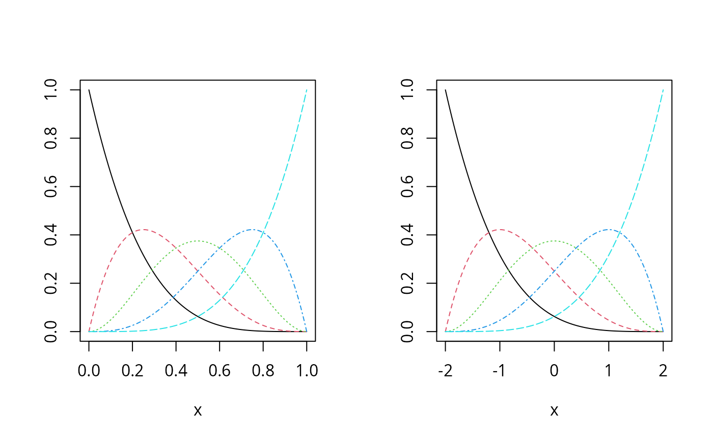
Returns generalized Bernstein polynomial basis functions of the given degree over the specified range.
Usage
bernsteinPoly(
  x,
  degree = 3,
  intercept = FALSE,
  Boundary.knots = NULL,
  derivs = 0L,
  integral = FALSE,
  ...
)

bpoly(
  x,
  degree = 3,
  intercept = FALSE,
  Boundary.knots = NULL,
  derivs = 0L,
  integral = FALSE,
  ...
)
Arguments
- x
The predictor variable taking values inside of the specified boundary. Missing values are allowed and will be returned as they are.
- degree
A nonnegative integer representing the degree of the polynomials.
- intercept
If
TRUE, the complete basis matrix will be returned. Otherwise, the first basis will be excluded from the output.- Boundary.knots
Boundary points at which to anchor the Bernstein polynomial basis. The default value is
NULLand the boundary knots is set internally to berange(x, na.rm = TRUE).- derivs
A nonnegative integer specifying the order of derivatives. The default value is
0Lfor Bernstein polynomial basis functions.- integral
A logical value. If
TRUE, the integrals of the Bernstein polynomials will be returned. The default value isFALSE.- ...
Optional arguments that are not used.
Value
A BernsteinPoly object that is essentially a numeric matrix
of dimension length(x) by degree + as.integer(intercept).
Details
The Bernstein polynomial basis functions are defined over the support from 0 to 1. The generalized Bernstein polynomial basis functions extend the support to any finite interval in the real line.
The function bpoly() is an alias to encourage the use in a model
formula.
Examples
library(splines2)

x1 <- seq.int(0, 1, 0.01)
x2 <- seq.int(- 2, 2, 0.01)

## Bernstein polynomial basis matrix over [0, 1]
bMat1 <- bernsteinPoly(x1, degree = 4, intercept = TRUE)

## generalized Bernstein polynomials basis over [- 2, 2]
bMat2 <- bernsteinPoly(x2, degree = 4, intercept = TRUE)

op <- par(mfrow = c(1, 2))
plot(bMat1)
plot(bMat2)


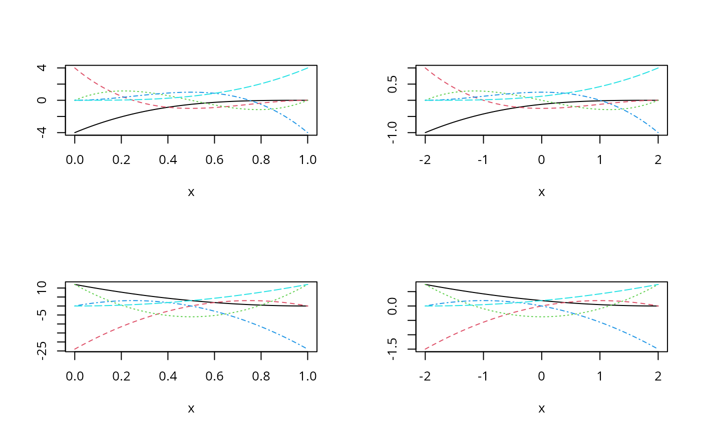
## the first and second derivative matrix
d1Mat1 <- bernsteinPoly(x1, degree = 4, derivs = 1, intercept = TRUE)
d2Mat1 <- bernsteinPoly(x1, degree = 4, derivs = 2, intercept = TRUE)
d1Mat2 <- bernsteinPoly(x2, degree = 4, derivs = 1, intercept = TRUE)
d2Mat2 <- bernsteinPoly(x2, degree = 4, derivs = 2, intercept = TRUE)

par(mfrow = c(2, 2))
plot(d1Mat1)
plot(d1Mat2)
plot(d2Mat1)
plot(d2Mat2)


## reset to previous plotting settings
par(op)

## or use the deriv method
all.equal(d1Mat1, deriv(bMat1))
#> [1] TRUE
all.equal(d2Mat1, deriv(bMat1, 2))
#> [1] TRUE

## the integrals
iMat1 <- bernsteinPoly(x1, degree = 4, integral = TRUE, intercept = TRUE)
iMat2 <- bernsteinPoly(x2, degree = 4, integral = TRUE, intercept = TRUE)
all.equal(deriv(iMat1), bMat1, check.attributes = FALSE)
#> [1] TRUE
all.equal(deriv(iMat2), bMat2, check.attributes = FALSE)
#> [1] TRUE