Natural Cubic Spline Basis for Polynomial Splines

Functions naturalSpline() and nsk() generate the natural cubic spline basis functions, the corresponding derivatives or integrals (from the left boundary knot). Both of them are different from splines::ns(). However, for a given model fitting procedure, using different variants of spline basis functions should result in identical prediction values. The coefficient estimates of the spline basis functions returned by nsk() are more interpretable compared to naturalSpline() or splines::ns() .

Usage

naturalSpline(
  x,
  df = NULL,
  knots = NULL,
  intercept = FALSE,
  Boundary.knots = NULL,
  trim = 0,
  derivs = 0L,
  integral = FALSE,
  ...
)

nsp(
  x,
  df = NULL,
  knots = NULL,
  intercept = FALSE,
  Boundary.knots = NULL,
  trim = 0,
  derivs = 0L,
  integral = FALSE,
  ...
)

nsk(
  x,
  df = NULL,
  knots = NULL,
  intercept = FALSE,
  Boundary.knots = NULL,
  trim = 0,
  derivs = 0L,
  integral = FALSE,
  ...
)

Arguments

x: The predictor variable. Missing values are allowed and will be returned as they are.
df: Degree of freedom that equals to the column number of returned matrix. One can specify df rather than knots, then the function chooses df - 1 - as.integer(intercept) internal knots at suitable quantiles of x ignoring missing values and those x outside of the boundary. Thus, df must be greater than or equal to 2. If internal knots are specified via knots, the specified df will be ignored.
knots: The internal breakpoints that define the splines. The default is NULL, which results in a basis for ordinary polynomial regression. Typical values are the mean or median for one knot, quantiles for more knots. For periodic splines, the number of knots must be greater or equal to the specified degree - 1.
intercept: If TRUE, the complete basis matrix will be returned. Otherwise, the first basis will be excluded from the output.
Boundary.knots: Boundary points at which to anchor the splines. By default, they are the range of x excluding NA. If both knots and Boundary.knots are supplied, the basis parameters do not depend on x. Data can extend beyond Boundary.knots. For periodic splines, the specified bounary knots define the cyclic interval.
trim: The fraction (0 to 0.5) of observations to be trimmed from each end of x before placing the default internal and boundary knots. This argument will be ignored if Boundary.knots is specified. The default value is 0 for backward compatibility, which sets the boundary knots as the range of x. If a positive fraction is specified, the default boundary knots will be equivalent to quantile(x, probs = c(trim, 1 - trim), na.rm = TRUE), which can be a more sensible choice in practice due to the existence of outliers. The default internal knots are placed within the boundary afterwards.
derivs: A nonnegative integer specifying the order of derivatives of natural splines. The default value is 0L for the spline basis functions.
integral: A logical value. The default value is FALSE. If TRUE, this function will return the integrated natural splines from the left boundary knot.
...: Optional arguments that are not used.

Value

A numeric matrix of length(x) rows and df

columns if df is specified or length(knots) + 1 + as.integer(intercept) columns if knots are specified instead. Attributes that correspond to the arguments specified are returned for usage of other functions in this package.

Details

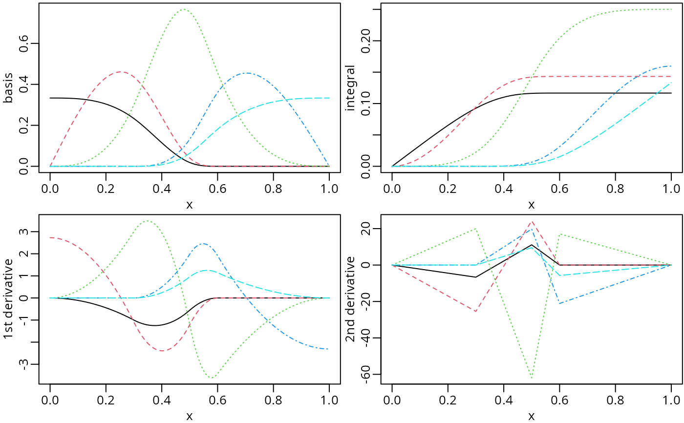
The constructed spline basis functions from naturalSpline() are nonnegative within boundary with the second derivatives being zeros at boundary knots. The implementation utilizes the close-form null space that can be derived from the recursive formula for the second derivatives of B-splines. The function nsp() is an alias of naturalSpline() to encourage the use in a model formula.

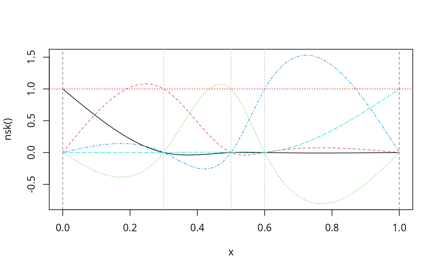
The function nsk() produces another variant of natural cubic spline matrix such that only one of the basis functions is nonzero and takes a value of one at every boundary and internal knot. As a result, the coefficients of the resulting fit are the values of the spline function at the knots, which makes it easy to interpret the coefficient estimates. In other words, the coefficients of a linear model will be the heights of the function at the knots if intercept = TRUE. If intercept = FALSE, the coefficients will be the change in function value between each knot. This implementation closely follows the function nsk() of the survival package (version 3.2-8). The idea corresponds directly to the physical implementation of a spline by passing a flexible strip of wood or metal through a set of fixed points, which is a traditional way to create smooth shapes for things like a ship hull.

The returned basis matrix can be obtained by transforming the corresponding B-spline basis matrix with the matrix H provided in the attribute of the returned object. Each basis is assumed to follow a linear trend for x outside of boundary. A similar implementation is provided by splines::ns, which uses QR decomposition to find the null space of the second derivatives of B-spline basis at boundary knots. See Supplementray Materials of Wang and Yan (2021) for a more detailed introduction.

Examples

library(splines2)

x <- seq.int(0, 1, 0.01)
knots <- c(0.3, 0.5, 0.6)

## naturalSpline()
nsMat0 <- naturalSpline(x, knots = knots, intercept = TRUE)
nsMat1 <- naturalSpline(x, knots = knots, intercept = TRUE, integral = TRUE)
nsMat2 <- naturalSpline(x, knots = knots, intercept = TRUE, derivs = 1)
nsMat3 <- naturalSpline(x, knots = knots, intercept = TRUE, derivs = 2)

op <- par(mfrow = c(2, 2), mar = c(2.5, 2.5, 0.2, 0.1), mgp = c(1.5, 0.5, 0))
plot(nsMat0, ylab = "basis")
plot(nsMat1, ylab = "integral")
plot(nsMat2, ylab = "1st derivative")
plot(nsMat3, ylab = "2nd derivative")

par(op) # reset to previous plotting settings

## nsk()
nskMat <- nsk(x, knots = knots, intercept = TRUE)
plot(nskMat, ylab = "nsk()", mark_knots = "all")
abline(h = 1, col = "red", lty = 3)


## use the deriv method
all.equal(nsMat0, deriv(nsMat1), check.attributes = FALSE)
#> [1] TRUE
all.equal(nsMat2, deriv(nsMat0))
#> [1] TRUE
all.equal(nsMat3, deriv(nsMat2))
#> [1] TRUE
all.equal(nsMat3, deriv(nsMat0, 2))
#> [1] TRUE

## a linear model example
fit1 <- lm(weight ~ -1 + nsk(height, df = 4, intercept = TRUE), data = women)
fit2 <- lm(weight ~ nsk(height, df = 3), data = women)

## the knots (same for both fits)
knots <- unlist(attributes(fit1$model[[2]])[c('Boundary.knots', 'knots')])

## predictions at the knot points
predict(fit1, data.frame(height = sort(unname(knots))))
#>        1        2        3        4 
#> 114.5595 127.9333 143.3219 163.6409 
unname(coef(fit1)) # equal to the coefficient estimates
#> [1] 114.5595 127.9333 143.3219 163.6409

## different interpretation when "intercept = FALSE"
unname(coef(fit1)[-1] - coef(fit1)[1]) # differences: yhat[2:4] - yhat[1]
#> [1] 13.37381 28.76248 49.08146
unname(coef(fit2))[-1]                 # ditto
#> [1] 13.37381 28.76248 49.08146