Compute Spline Function for Given Coefficients

Returns the spline function (with the specified coefficients) or evaluate the basis functions at the specified x if the coefficients are not specified.

Usage

# S3 method for class 'BSpline'
predict(object, newx = NULL, coef = NULL, ...)

# S3 method for class 'MSpline'
predict(object, newx = NULL, coef = NULL, ...)

# S3 method for class 'ISpline'
predict(object, newx = NULL, coef = NULL, ...)

# S3 method for class 'CSpline'
predict(object, newx = NULL, coef = NULL, ...)

# S3 method for class 'BernsteinPoly'
predict(object, newx = NULL, coef = NULL, ...)

# S3 method for class 'NaturalSpline'
predict(object, newx = NULL, coef = NULL, ...)

# S3 method for class 'NaturalSplineK'
predict(object, newx = NULL, coef = NULL, ...)

Arguments

object: Spline objects produced by the splines2 package.
newx: The x values at which evaluations are required. If it is NULL (by default), the original x used to create the spline object will be used.
coef: A numeric vector specifying the coefficients of the spline basis functions. If it is NULL (by default), the spline basis functions will be returned. Otherwise, the resulting spline function will be returned.
...: Other options passed to the corresponding function that constructs the input object. For example, the additional options will be passed to bSpline() for a BSpline object.

Value

The function returns the spline basis functions with the new values of x if coef is not specified. Otherwise, the function returns the resulting spline function (or its derivative if derivs is specified as a positive integer through ...).

Examples

library(splines2)

x <- seq.int(0, 1, 0.2)
knots <- c(0.3, 0.5, 0.6)
newx <- seq.int(0.1, 0.9, 0.2)

## Cubic B-spline basis functions
bs_mat <- bSpline(x, knots = knots)

## compute the B-spline basis functions at new x
predict(bs_mat, newx)
#>              1          2           3            4        5        6
#> [1,] 0.5392593 0.15333333 0.011111111 0.000000e+00 0.000000 0.000000
#> [2,] 0.1600000 0.54000000 0.300000000 4.072784e-48 0.000000 0.000000
#> [3,] 0.0000000 0.05555556 0.753968254 1.904762e-01 0.000000 0.000000
#> [4,] 0.0000000 0.00000000 0.192857143 5.496429e-01 0.241875 0.015625
#> [5,] 0.0000000 0.00000000 0.007142857 1.203571e-01 0.450625 0.421875

## compute the B-spline function for the specified coefficients
beta <- runif(ncol(bs_mat))
predict(bs_mat, coef = beta)
#> [1] 0.0000000 0.5708690 0.7091796 0.5499994 0.5144477 0.8802465

## compute the first derivative of the B-spline function
predict(bs_mat, coef = beta, derivs = 1)
#> [1]  2.3872603  2.4854897 -0.9511306 -0.4309568  0.4505289  3.5825490
## or equivalently
predict(deriv(bs_mat), coef = beta)
#> [1]  2.3872603  2.4854897 -0.9511306 -0.4309568  0.4505289  3.5825490

## compute the second derivative
predict(bs_mat, coef = beta, derivs = 2)
#> [1]  13.030248 -12.047953  -7.510345  -1.218908  10.033764  21.286437
## or equivalently
predict(deriv(bs_mat, derivs = 2), coef = beta)
#> [1]  13.030248 -12.047953  -7.510345  -1.218908  10.033764  21.286437

## compute the integral
predict(bs_mat, coef = beta, integral = TRUE)
#> [1] 0.00000000 0.05675947 0.19745372 0.32047678 0.42398320 0.55301255
## or equivalently
predict(update(bs_mat, integral = TRUE), coef = beta)
#> [1] 0.00000000 0.05675947 0.19745372 0.32047678 0.42398320 0.55301255

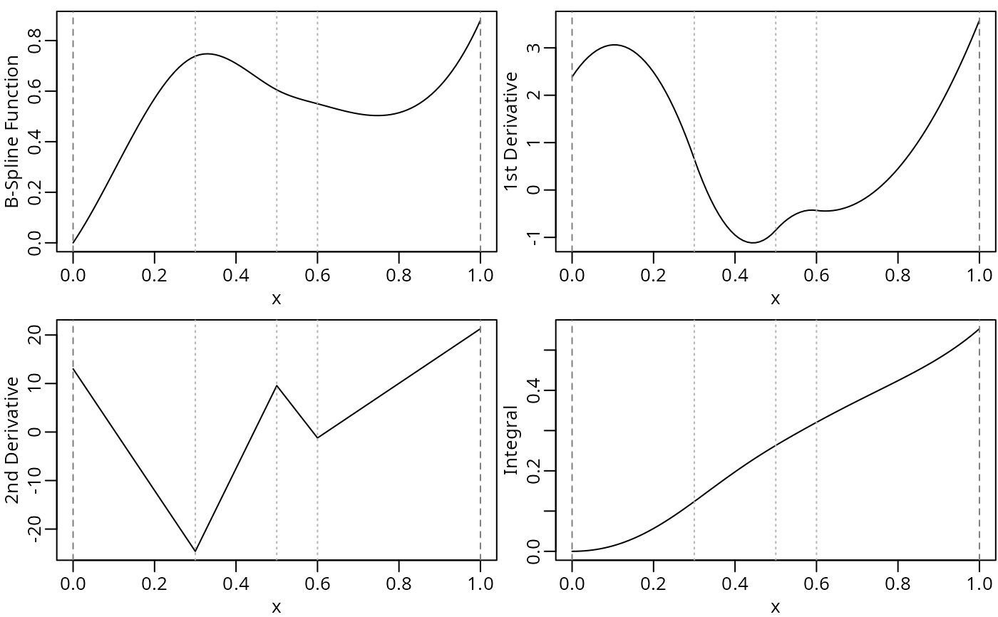
## visualize
op <- par(mfrow = c(2, 2), mar = c(2.5, 2.5, 0.5, 0.1), mgp = c(1.5, 0.5, 0))
plot(bs_mat, coef = beta, ylab = "B-Spline Function", mark_knots = "all")
plot(deriv(bs_mat), coef = beta, ylab = "1st Derivative", mark_knots = "all")
plot(deriv(bs_mat, derivs = 2), coef = beta,
     ylab = "2nd Derivative", mark_knots = "all")
plot(update(bs_mat, integral = TRUE), coef = beta,
     ylab = "Integral", mark_knots = "all")

par(op)