B-Spline Basis for Polynomial Splines

Generates the spline basis matrix for B-splines representing the family of piecewise polynomials with the specified interior knots, degree, and boundary knots, evaluated at the values of x.

Usage

bSpline(
  x,
  df = NULL,
  knots = NULL,
  degree = 3L,
  intercept = FALSE,
  Boundary.knots = NULL,
  periodic = FALSE,
  derivs = 0L,
  integral = FALSE,
  warn.outside = getOption("splines2.warn.outside", TRUE),
  ...
)

ibs(
  x,
  df = NULL,
  knots = NULL,
  degree = 3,
  intercept = FALSE,
  Boundary.knots = NULL,
  ...
)

dbs(
  x,
  derivs = 1L,
  df = NULL,
  knots = NULL,
  degree = 3,
  intercept = FALSE,
  Boundary.knots = NULL,
  ...
)

bsp(
  x,
  df = NULL,
  knots = NULL,
  degree = 3L,
  intercept = FALSE,
  Boundary.knots = NULL,
  periodic = FALSE,
  derivs = 0L,
  integral = FALSE,
  warn.outside = getOption("splines2.warn.outside", TRUE),
  ...
)

Arguments

x: The predictor variable. Missing values are allowed and will be returned as they are.
df: Degree of freedom that equals to the column number of the returned matrix. One can specify df rather than knots, then the function chooses df - degree - as.integer(intercept) internal knots at suitable quantiles of x ignoring missing values and those x outside of the boundary. For periodic splines, df - as.integer(intercept) internal knots will be chosen at suitable quantiles of x relative to the beginning of the cyclic intervals they belong to (see Examples) and the number of internal knots must be greater or equal to the specified degree - 1. If internal knots are specified via knots, the specified df will be ignored.
knots: The internal breakpoints that define the splines. The default is NULL, which results in a basis for ordinary polynomial regression. Typical values are the mean or median for one knot, quantiles for more knots. For periodic splines, the number of knots must be greater or equal to the specified degree - 1. Duplicated internal knots are not allowed.
degree: A nonnegative integer specifying the degree of the piecewise polynomial. The default value is 3 for cubic splines. Zero degree is allowed for piecewise constant basis functions.
intercept: If TRUE, the complete basis matrix will be returned. Otherwise, the first basis will be excluded from the output.
Boundary.knots: Boundary points at which to anchor the splines. By default, they are the range of x excluding NA. If both knots and Boundary.knots are supplied, the basis parameters do not depend on x. Data can extend beyond Boundary.knots. For periodic splines, the specified bounary knots define the cyclic interval.
periodic: A logical value. If TRUE, the periodic splines will be returned. The default value is FALSE.
derivs: A nonnegative integer specifying the order of derivatives of splines basis function. The default value is 0.
integral: A logical value. If TRUE, the corresponding integrals of spline basis functions will be returned. The default value is FALSE. For periodic splines, the integral of each basis is integrated from the left boundary knot.
warn.outside: A logical value indicating if a warning should be thrown out when any x is outside the boundary. This option can also be set through options("splines2.warn.outside") after the package is loaded.
...: Optional arguments that are not used.

Value

A numeric matrix of length(x) rows and df columns if df is specified. If knots are specified instead, the output matrix will consist of length(knots) + degree + as.integer(intercept) columns if periodic = FALSE, or length(knots) + as.integer(intercept) columns if periodic = TRUE. Attributes that correspond to the arguments specified are returned for usage of other functions in this package.

Details

This function extends the bs() function in the splines package for B-spline basis functions by allowing piecewise constant (left-closed and right-open except on the right boundary) spline basis of degree zero. In addition, the function provides derivatives or integrals of the B-spline basis functions when one specifies the arguments derivs or integral appropriately. The function constructs periodic B-splines when periodic is TRUE. All the implementations are based on the closed-form recursion formula following De Boor (1978) and Wang and Yan (2021).

The functions ibs() and dbs() are provided for convenience. The former provides the integrals of B-splines and is equivalent to bSpline() with integral = TRUE. The latter produces the derivatives of given order of B-splines and is equivalent to bSpline() with default derivs = 1. The function bsp() is an alias of to encourage the use in a model formula.

References

De Boor, Carl. (1978). A practical guide to splines. Vol. 27. New York: Springer-Verlag.

Wang, W., & Yan, J. (2021). Shape-restricted regression splines with R package splines2. Journal of Data Science, 19(3),498–517.

Examples

library(splines2)

set.seed(1)
x <- runif(100)
knots <- c(0.3, 0.5, 0.6) # internal knots

## cubic B-splines
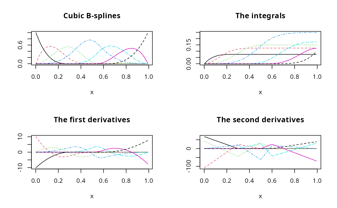
bsMat <- bSpline(x, knots = knots, degree = 3, intercept = TRUE)
ibsMat <- update(bsMat, integral = TRUE) # the integrals
d1Mat <- deriv(bsMat)                    # the 1st derivaitves
d2Mat <- deriv(bsMat, 2)                 # the 2nd derivaitves

op <- par(mfrow = c(2, 2), mar = c(2.5, 2.5, 0.2, 0.1), mgp = c(1.5, 0.5, 0))
plot(bsMat, ylab = "Cubic B-splines")
plot(ibsMat, ylab = "The integrals")
plot(d1Mat, ylab = "The 1st derivatives")
plot(d2Mat, ylab = "The 2nd derivatives")


## evaluate at new values
predict(bsMat, c(0.125, 0.801))
#>              1         2         3          4         5         6         7
#> [1,] 0.2276364 0.5596808 0.1956893 0.01699357 0.0000000 0.0000000 0.0000000
#> [2,] 0.0000000 0.0000000 0.0000000 0.05216125 0.3495278 0.4634015 0.1349094

## periodic B-splines
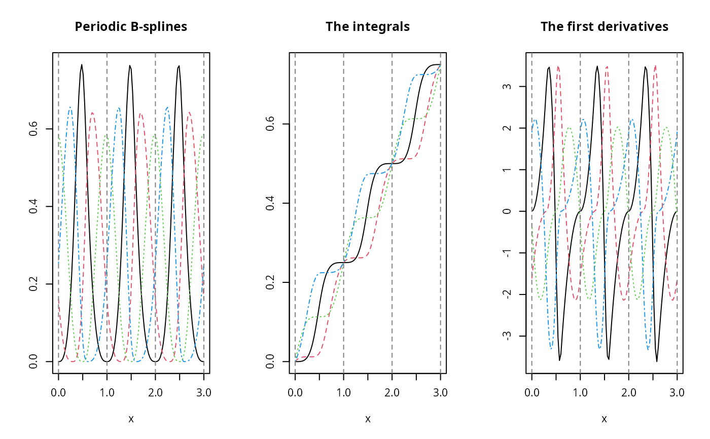
px <- seq(0, 3, 0.01)
pbsMat <- bSpline(px, knots = knots, Boundary.knots = c(0, 1),
                  intercept = TRUE, periodic = TRUE)
ipMat <- update(pbsMat, integral = TRUE)
dpMat <- deriv(pbsMat)
dp2Mat <- deriv(pbsMat, 2)

plot(pbsMat, ylab = "Periodic B-splines", mark_knots = "b")
plot(ipMat, ylab = "The integrals", mark_knots = "b")
plot(dpMat, ylab = "The 1st derivatives", mark_knots = "b")
plot(dp2Mat, ylab = "The 2nd derivatives", mark_knots = "b")

par(op) # reset to previous plotting settings