An S4 class generic function that returns the mean cumulative function (MCF) estimates from a fitted model or returns the nonparametric MCF estimates (by Nelson-Aalen estimator or Cook-Lawless cumulative sample mean estimator) from the sample data.
Usage
mcf(object, ...)

# S4 method for class 'formula'
mcf(
  object,
  data,
  subset,
  na.action,
  variance = c("LawlessNadeau", "Poisson", "bootstrap", "CSV", "none"),
  logConfInt = FALSE,
  adjustRiskset = TRUE,
  level = 0.95,
  control = list(),
  ...
)

# S4 method for class 'rateReg'
mcf(
  object,
  newdata,
  groupName,
  groupLevels,
  level = 0.95,
  na.action,
  control = list(),
  ...
)
Arguments
- object
An object used to dispatch a method.
- ...
Other arguments for future usage.
- data
A data frame, list or environment containing the variables in the model. If not found in data, the variables are taken from
environment(formula), usually the environment from which the function is called.- subset
An optional vector specifying a subset of observations to be used in the fitting process.
- na.action
A function that indicates what should the procedure do if the data contains
NAs. The default is set by the na.action setting ofoptions. The "factory-fresh" default isna.omit. Other possible values inlcudena.fail,na.exclude, andna.pass.help(na.fail)for details.- variance
A character specifying the method for variance estimates. The available options are
"LawlessNadeau"(the default) for Lawless and Nadeau (1995) method,"Poisson"for Poisson process method,"bootstrap"for bootstrap method,"CSV"for variance estimates of the corresponding cumulative sample mean function (CSM) by the cumulative sample variance method (Cook and Lawless, 2007), and"none"for no variance estimates. Partial matching on the names is allowed.- logConfInt
A logical value. If
FALSE(the default), the confidence interval are constructed based on the normality of the MCF estimates. Otherwise, the confidence intervals of given level are constucted based on the normality of logarithm of the MCF estimates.- adjustRiskset
A logical value indicating whether to adjust the size of risk-set. If
TRUEby default, the size of risk-set will be adjusted based on at-risk indicators and Nelson-Aalen estimator will be returned. Otherwise, the cumulative sample mean (CSM) function given by Cook and Lawless (2007) will be returned without adjustment on size of risk-set.- level
An optional numeric value indicating the confidence level required. The default value is 0.95.
- control
An optional named list specifying other options. For
rateRegobject, it can be used to specify the time grid where the MCF is estimated. The available named elements are given as follows:grid: The time grid where MCF is estimated. A dense grid is suggested for further using the plot method.length.out: The length of grid points. The dafault value is 1,000.from: The starting point of grid. The default value is the left boundary knots (forrateRegobject).to: The endpoint of grid. The default value is the right boundary knots (forrateRegobject).
The option
length.out,from,towill be ignored ifgridis specified directly. Otherwise, the grid will be generated by functionseq.intwith specifiedfrom,toandlength.out.For formula method, the available named elements are given as follows:
B: The number of bootstrap replicates for using bootstrap method for variance estimates of sample MCF estimates. The default value is 200.se.method: The method used for SE estimates for bootstrap. The available methods include"sample.se"(the default) and"normality". The former takes the sample SE of point estimates from bootstrap samples; The latter estimates SE based on interquantile and normality assumption.ci.method: The method used for confidence interval (CI) for bootstrap. The available options include"normality"(the default) and"percentile". The former estimates the CI based on SE estimates and normality assumption; The latter takes percentiles of the bootstrap estimates.keep.data: A logical value specifying whether to keep the processed data in the output object. IfTRUE(the default), the processed data will be kept in the output and available for later usage. Otherwise, an empty data frame object will be returned in thedataslot.FALSEmay be set when the memory consumption is of concern and we only need MCF estimates. For example, the functionmcfDiffandmcfDiff.testwill not be applicable for themcf.formulaobject with an emptydataslot.verbose: A logical value. The default value isTRUE. IfFALSE, possible data checking messages (not including warnings or errors) will be suppressed.
- newdata
An optional data frame. If specified, the data frame should have the same column names as the covariate names appearing in the formula of original fitting.
- groupName
An optional length-one charactor vector to specify the name for grouping each unique row in
newdata, such as "gender" for "male" and "female". The default value is "Group".- groupLevels
An optional charactor vector to specify the levels for each unique row in
newdata, such as "treatment" and "control". The default values are"Level"followed by a numeric sequence with length of number of levels.
Value
A mcf.formula or mcf.rateReg object.
A brief description of the slots of a mcf.formula object is given as
follows:
formula: Model Formula.data: Processed data based on the model formula or an empty data frame ifkeep.datais set to beFALSE.MCF: A data frame containing estimates for sample MCF.origin: Time origins.multiGroup: A logical value indicating whether MCF is estimated for different groups respectively.logConfInt: A logical value indicating whether the variance estimates are based on the normality of logarithm of the MCF estimates.level: Confidence level specified.
Most slots of a mcf.rateReg object are inherited from the input
rateReg object. A brief description of other slots is given as
follows:
newdata: Given dataset used to estimate MCF.MCF: A data frame containing MCF estimates.level: Confidence level specified.na.action: The way handling missing values.control: The control list.multiGroup: A logical value indicating whether MCF is estimated for different groups respectively.
Details
For formula object with Recur object as response, the
covariate specified at the right hand side of the formula should be either
1 or any "linear" conbination of categorical variable in the data.
The former computes the overall sample MCF. The latter computes the sample
MCF for each level of the combination of the categorical variable(s)
specified, respectively.
The MCF estimates are computed on each unique time point of the sample data.
By default, the size of risk set is adjusted over time based on the at-risk
indicators, which results in the Nelson-Aalen nonparametric estimator
(Nelson 2003). If the size of risk set remains a constant (total number of
processes) over time (specified by adjustRiskset = FALSE), the
cumulative sample mean (CSM) function introduced in Chapter 1 of Cook and
Lawless (2007) will be computed instead. The point estimate of sample MCF
at each time point does not assume any particular underlying model. The
variance estimates at each time point is computed following the Lawless and
Nadeau method (LawLess and Nadeau 1995), the Poisson process method, or the
bootstrap methods. The approximate confidence intervals are provided as
well, which are constructed based on the asymptotic normality of the MCF
itself (by default) or the logarithm of MCF.
For rateReg object, mcf estimates the baseline MCF and its
confidence interval at each time grid if argument newdata is not
specified. Otherwise, mcf estimates MCF and its confidence interval
for the given newdata based on Delta-method.
References
Cook, R. J., and Lawless, J. (2007). The statistical analysis of recurrent events, Springer Science & Business Media.
Lawless, J. F. and Nadeau, C. (1995). Some Simple Robust Methods for the Analysis of Recurrent Events. Technometrics, 37, 158–168.
Nelson, W. B. (2003). Recurrent Events Data Analysis for Product Repairs, Disease Recurrences, and Other Applications (Vol. 10). SIAM.
See also
rateReg for model fitting;
mcfDiff for comparing two-sample MCFs.
plot-method for plotting MCF.
Examples
library(reda)
### sample MCF
## Example 1. valve-seat data
## the default variance estimates by Lawless and Nadeau (1995) method
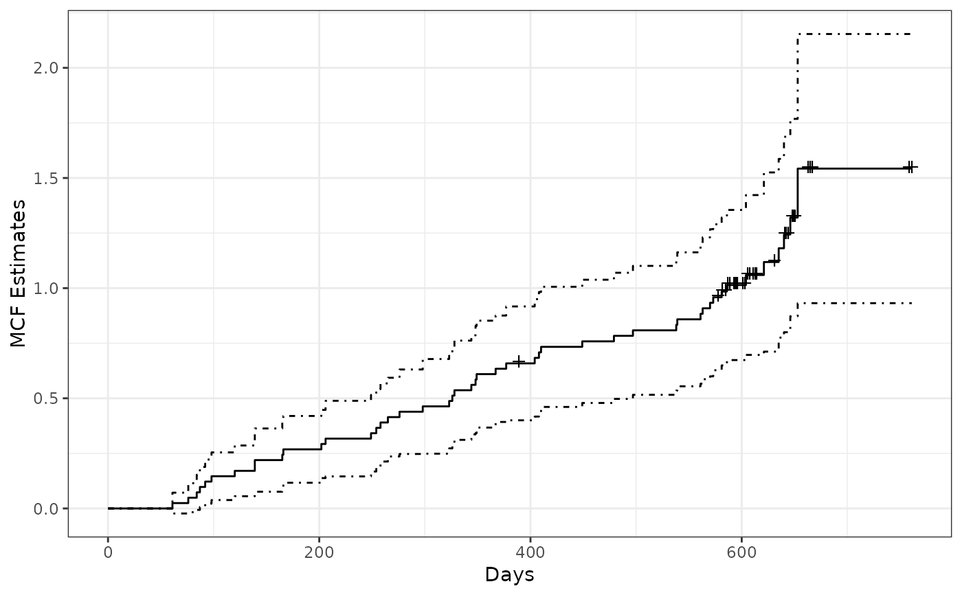
valveMcf0 <- mcf(Recur(Days, ID, No.) ~ 1, data = valveSeats)
plot(valveMcf0, conf.int = TRUE, mark.time = TRUE, addOrigin = TRUE) +
ggplot2::xlab("Days") + ggplot2::theme_bw()
 ## variance estimates following Poisson process model
valveMcf1 <- mcf(Recur(Days, ID, No.) ~ 1,
data = valveSeats, variance = "Poisson")
## variance estimates by bootstrap method (with 1,000 bootstrap samples)
set.seed(123)
valveMcf2 <- mcf(Recur(Days, ID, No.) ~ 1,
data = valveSeats, variance = "bootstrap",
control = list(B = 200))
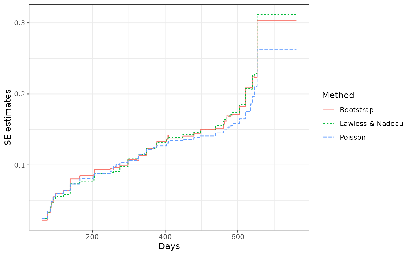
## comparing the variance estimates from different methods
library(ggplot2)
ciDat <- rbind(cbind(valveMcf0@MCF, Method = "Lawless & Nadeau"),
cbind(valveMcf1@MCF, Method = "Poisson"),
cbind(valveMcf2@MCF, Method = "Bootstrap"))
ggplot(ciDat, aes(x = time, y = se)) +
geom_step(aes(color = Method, linetype = Method)) +
xlab("Days") + ylab("SE estimates") + theme_bw()
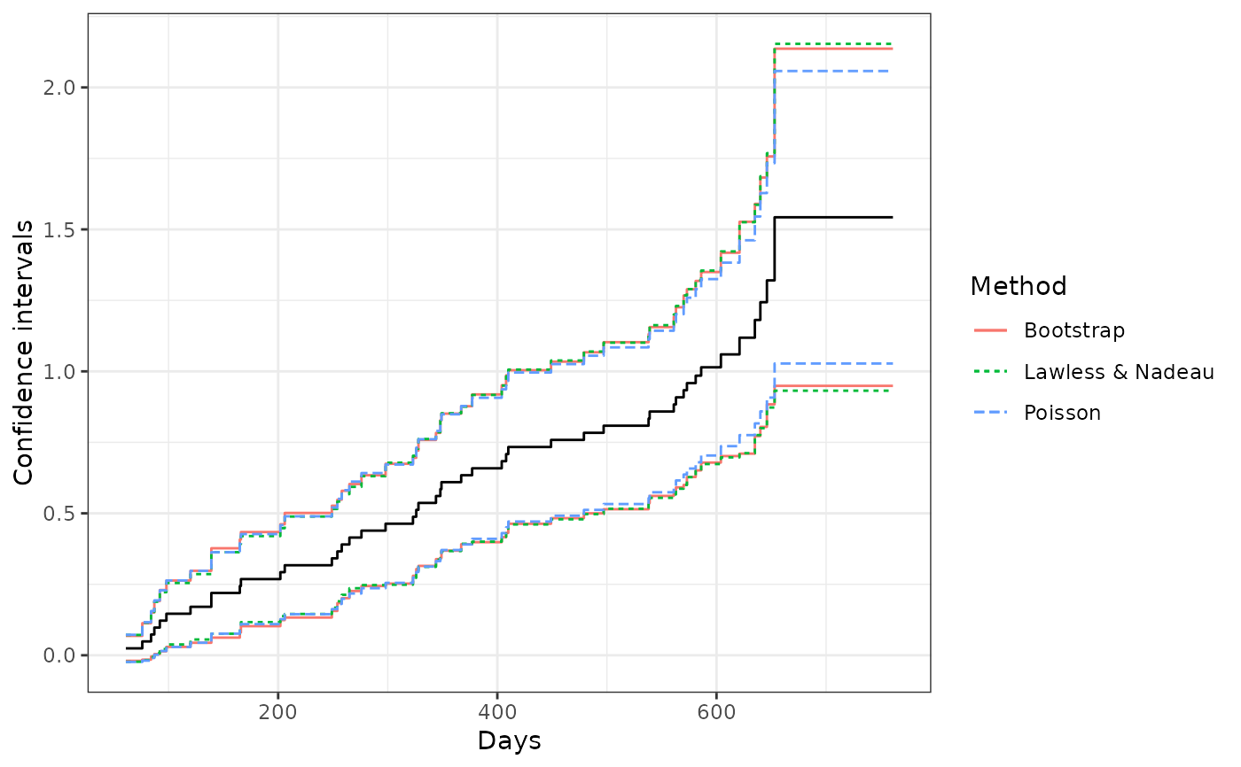
 ## comparing the confidence interval estimates from different methods
ggplot(ciDat, aes(x = time)) +
geom_step(aes(y = MCF)) +
geom_step(aes(y = lower, color = Method, linetype = Method)) +
geom_step(aes(y = upper, color = Method, linetype = Method)) +
xlab("Days") + ylab("Confidence intervals") + theme_bw()
 ## Example 2. the simulated data
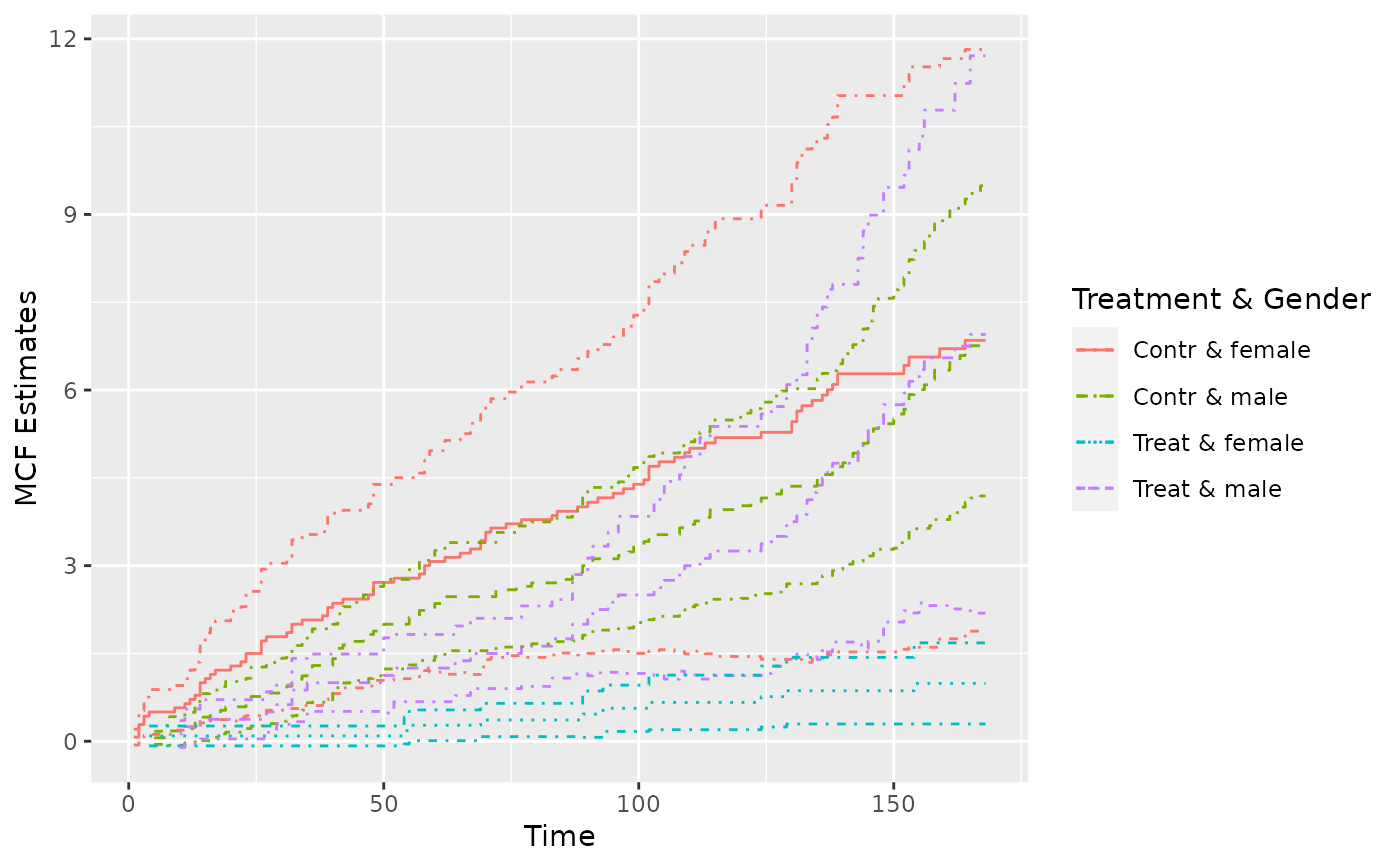
simuMcf <- mcf(Recur(time, ID, event) ~ group + gender,
data = simuDat, ID %in% 1 : 50)
plot(simuMcf, conf.int = TRUE, lty = 1 : 4,
legendName = "Treatment & Gender")
 ### estimate MCF difference between two groups
## one sample MCF object of two groups
mcf0 <- mcf(Recur(time, ID, event) ~ group, data = simuDat)
## two-sample pseudo-score tests
mcfDiff.test(mcf0)
#> Two-Sample Pseudo-Score Tests:
#> Statistic Variance Chisq DF Pr(>Chisq)
#> Constant Weight 52.5855 670.1014 4.1266 1 0.042214 *
#> Linear Weight 35.7687 158.9869 8.0472 1 0.004557 **
#> ---
#> Signif. codes: 0 ‘***’ 0.001 ‘**’ 0.01 ‘*’ 0.05 ‘.’ 0.1 ‘ ’ 1
#>
#> Variance Estimator: robust
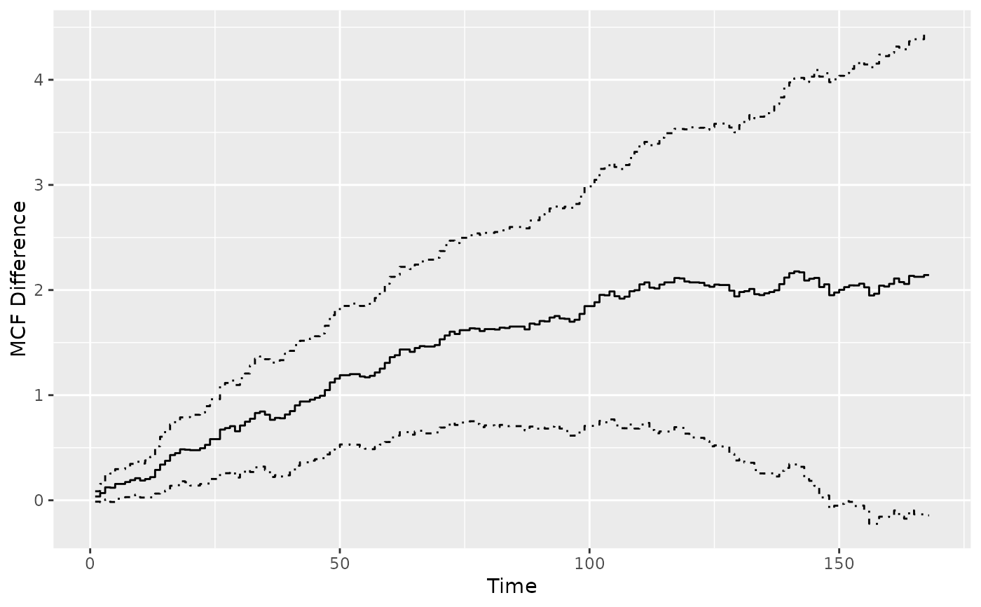
## difference estimates over time
mcf0_diff <- mcfDiff(mcf0, testVariance = "none")
plot(mcf0_diff)
 ## or explicitly ask for the difference of two sample MCF
mcf1 <- mcf(Recur(time, ID, event) ~ 1, data = simuDat,
subset = group %in% "Contr")
mcf2 <- mcf(Recur(time, ID, event) ~ 1, data = simuDat,
subset = group %in% "Treat")
## perform two-sample tests and estimate difference at the same time
mcf12_diff1 <- mcfDiff(mcf1, mcf2)
mcf12_diff2 <- mcf1 - mcf2 # or equivalently using the `-` method
stopifnot(all.equal(mcf12_diff1, mcf12_diff2))
mcf12_diff1
#> Call:
#> mcfDiff(mcf1 = mcf1, mcf2 = mcf2)
#>
#> Two-Sample Pseudo-Score Tests:
#> Statistic Variance Chisq DF Pr(>Chisq)
#> Constant Weight 52.5855 670.1014 4.1266 1 0.042214 *
#> Linear Weight 35.7687 158.9869 8.0472 1 0.004557 **
#> ---
#> Signif. codes: 0 ‘***’ 0.001 ‘**’ 0.01 ‘*’ 0.05 ‘.’ 0.1 ‘ ’ 1
#>
#> Variance Estimator: robust
plot(mcf12_diff1)
 ### For estimated MCF from a fitted model,
### see examples given in function rateReg.